Forces Through the Network
A Field-Theoretic View of Transmission
Bottom line up front
Central-bank policy, supply-chain shocks, political shifts, and contagion events all reach the real economy through the same intermediate object: a network of beliefs, contracts, and flows that behaves more like a field than a balance sheet. This document treats transmission as the central object of meso-economics.
Four claims organize what follows.
One. Transmission is not a black box; it is a field. Signals propagate through the Shimmer with measurable diffusion, decay, and source terms. The same equation describes a Fed announcement, a viral fear, and a supply-chain pulse.
Two. The same signal produces qualitatively different outcomes depending on the network it crosses. Topology and coupling strength --- random vs scale-free vs small-world, loose vs tight --- determine whether a shock damps out, propagates cleanly, or cascades.
Three. Distortion is the rule, not the exception. Multi-tier networks amplify signals (bullwhip). Belief contagion follows SIR dynamics with a measurable R₀. Response curves are S-shaped, not linear. Above critical coupling, small inputs produce large outputs.
Four. The aggregates we measure --- inflation, GDP, the credit cycle --- are emergent fields, not primary objects. They are statistical fingerprints of millions of micro decisions coordinated through the Shimmer. Treating them as primary makes monetary policy harder than it needs to be.
Ten historical cases validate the framework across the full design space --- from Volcker 1979 (slow tight credit channel) to ECB OMT 2012 (pure forward guidance) to Suez 2021 (physical supply-chain choke).
The ten expert lenses
Each section in this document brings one or more of the following perspectives to bear on transmission. None is sufficient alone. Together they cover the design space MECE.
1. Monetary economist. Mishkin (1995); Bernanke & Gertler (1995). The textbook transmission channels --- interest rate, credit, asset price, exchange rate, expectations. The catalogue of mechanisms.
2. Network scientist. Watts & Strogatz (1998); Barabási & Albert (1999). The topology of the medium --- random graphs, scale-free networks, small-world structures, percolation. The shape of the wires.
3. Behavioral economist. Akerlof & Shiller (2009); Kahneman (2011). Animal spirits, narratives, sentiment cascades, heuristic substitution. Why beliefs do not respect Bayesian updating.
4. Supply-chain operations researcher. Sterman (1989, 2000); Lee, Padmanabhan & Whang (1997). The bullwhip effect. Information distortion through multi-tier inventory networks. The mechanics of overshoot.
5. Complex-systems physicist. Bak, Tang & Wiesenfeld (1987); Sornette (2003). Self-organized criticality, phase transitions, power-law response. Why "normal" and "crisis" are different regimes of the same system.
6. Information theorist. Shannon (1948). Signal, noise, bandwidth, latency. The Shannon capacity of an economic channel. The cost of forwarding belief.
7. Epidemiologist. Kermack & McKendrick (1927); Anderson & May (1991). SIR/SEIR dynamics. The basic reproduction number R₀. Why belief contagion looks like disease contagion.
8. Control theorist / coupled oscillator. Strogatz (2003). Synchronization, phase-locking, tight vs loose coupling. The difference between a damped harmonic and a runaway feedback.
9. Market-microstructure financial economist. Kyle (1985); Glosten & Milgrom (1985). Liquidity propagation, adverse selection, the depth of order books. How a signal becomes a price.
10. Macro-historian. Kindleberger (1978); Reinhart & Rogoff (2009). Pattern recognition across crises. Why "this time is different" rarely is. The case-study base on which everything else gets validated.
Part one: Mechanism
How signal moves
How does a Fed press release at 2pm Tuesday become a smaller grocery cart in November? The honest answer is that it travels through a network of belief-holders, with each hop introducing delay and signal loss. Part One opens the mechanism.
The monetary economist's catalogue (Mishkin 1995) names six transmission channels but does not formalize how any of them propagate. The meso-economic move is to treat all six as instances of the same underlying field dynamic: a signal injected at one node, diffusing across coupled neighbors, decaying as it travels, and arriving at the periphery as a behavioral response.
The cascade unfolds in six stages, each on a different timescale. Trading desks reprice within minutes, because they are the network's fast layer --- densely connected, instrument-coupled, and watching the same screens. Banks revise lending guidelines within days, because internal credit committees are slower than dealer desks but faster than firms. Firms reset investment plans within weeks, because capital-budgeting cycles are quarterly. Households change their spending within months, because spending habits have inertia. Inflation and GDP respond within six to eighteen months, because they are aggregate statistical fingerprints that take many micro adjustments to register.
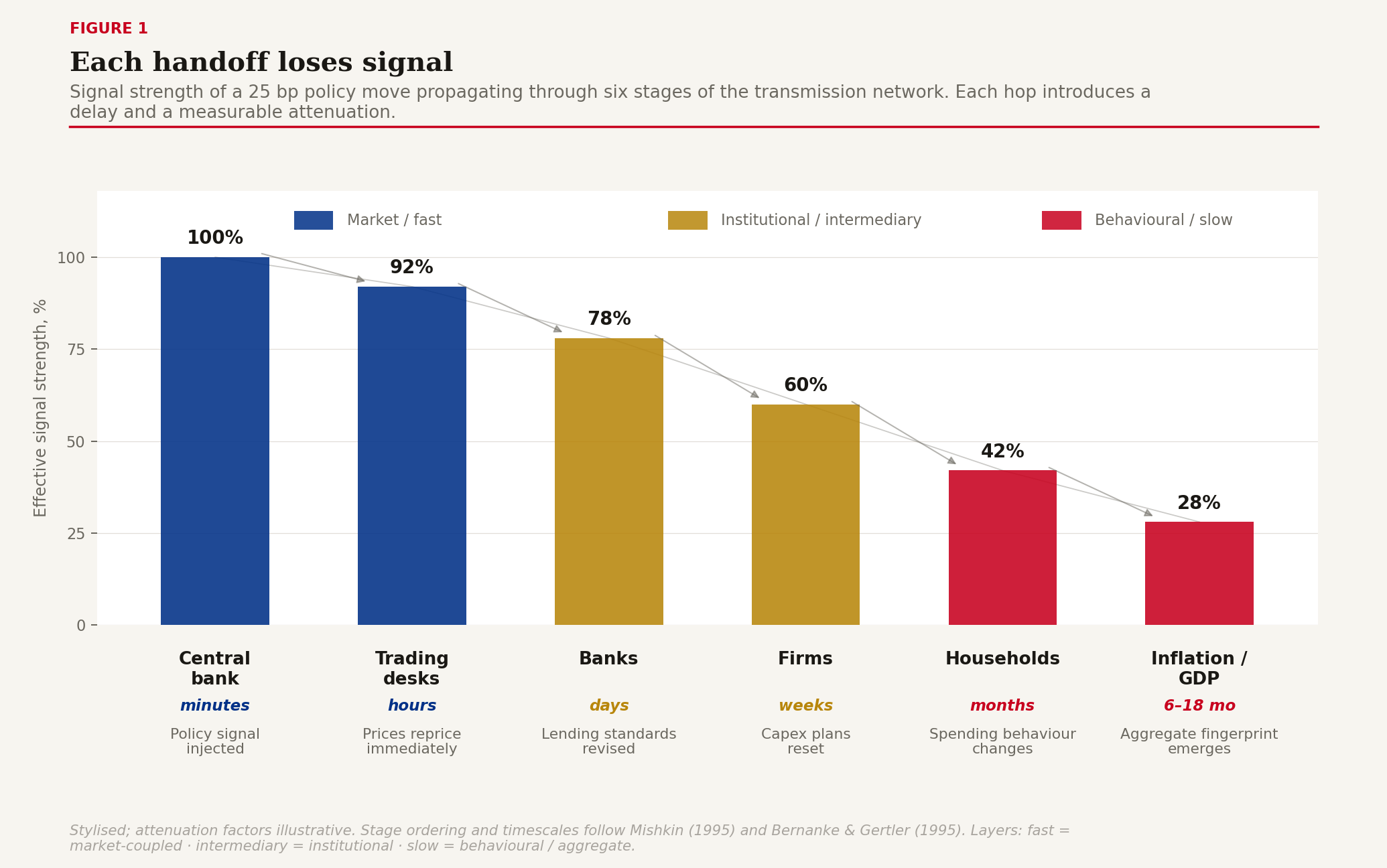
Figure 1: The six-stage transmission cascade --- each step a belief, each step a delay. Signal-strength bars show attenuation at each hop. Layer tags identify fast / intermediary / slow layers.
Topology determines speed and resilience. A random network has uniform short paths and high diversity; signals reach everyone quickly but no single node controls the propagation. A scale-free network --- like the banking system viewed through the Fed --- is hub-and-spoke; signals travel fast from the hub but the whole system is fragile to hub failure. A small-world network --- local clusters connected by a few long shortcuts --- combines speed and resilience and is the topology most real economic networks actually exhibit.
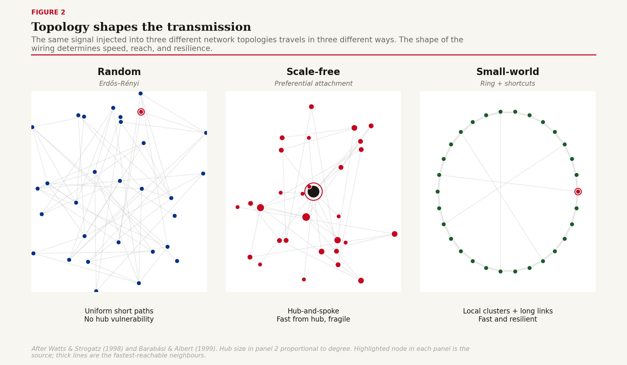
Figure 2: Three network topologies, three transmission speeds. Random, scale-free, and small-world, with example domains beneath each.
The signal itself decomposes into three forces. Diffusion spreads it across the network at rate D. Decay erases it at rate λ. The source S keeps re-injecting it. The field equation is mathematically identical to the heat equation in physics, which is not metaphor --- it is the same operator on a different graph.
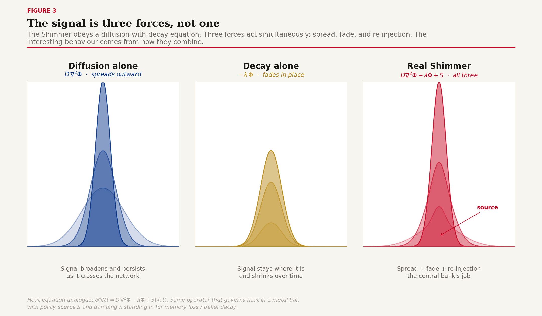
Figure 3: Decomposing the field. Three panels: diffusion alone broadens and persists; decay alone shrinks in place; the real Shimmer needs both, plus source. ∂Φ/∂t = D∇²Φ − λΦ + S.
The decisive variable is coupling --- the dynamic-systems property that determines whether two parts of the network move independently or in lockstep. Loose coupling is what makes diversified equity markets resilient; tight coupling is what makes derivatives books cascade. The interesting fact is that coupling strength interacts with speed: a fast loose network adjusts gracefully, a fast tight network produces cascade or contagion, a slow loose network is resilient but stagnant, and a slow tight network accumulates fragility silently for years until something snaps. Most banking-system fragility lives in the slow-tight quadrant. Most pandemic-style supply-chain collapse lives in the fast-tight quadrant.
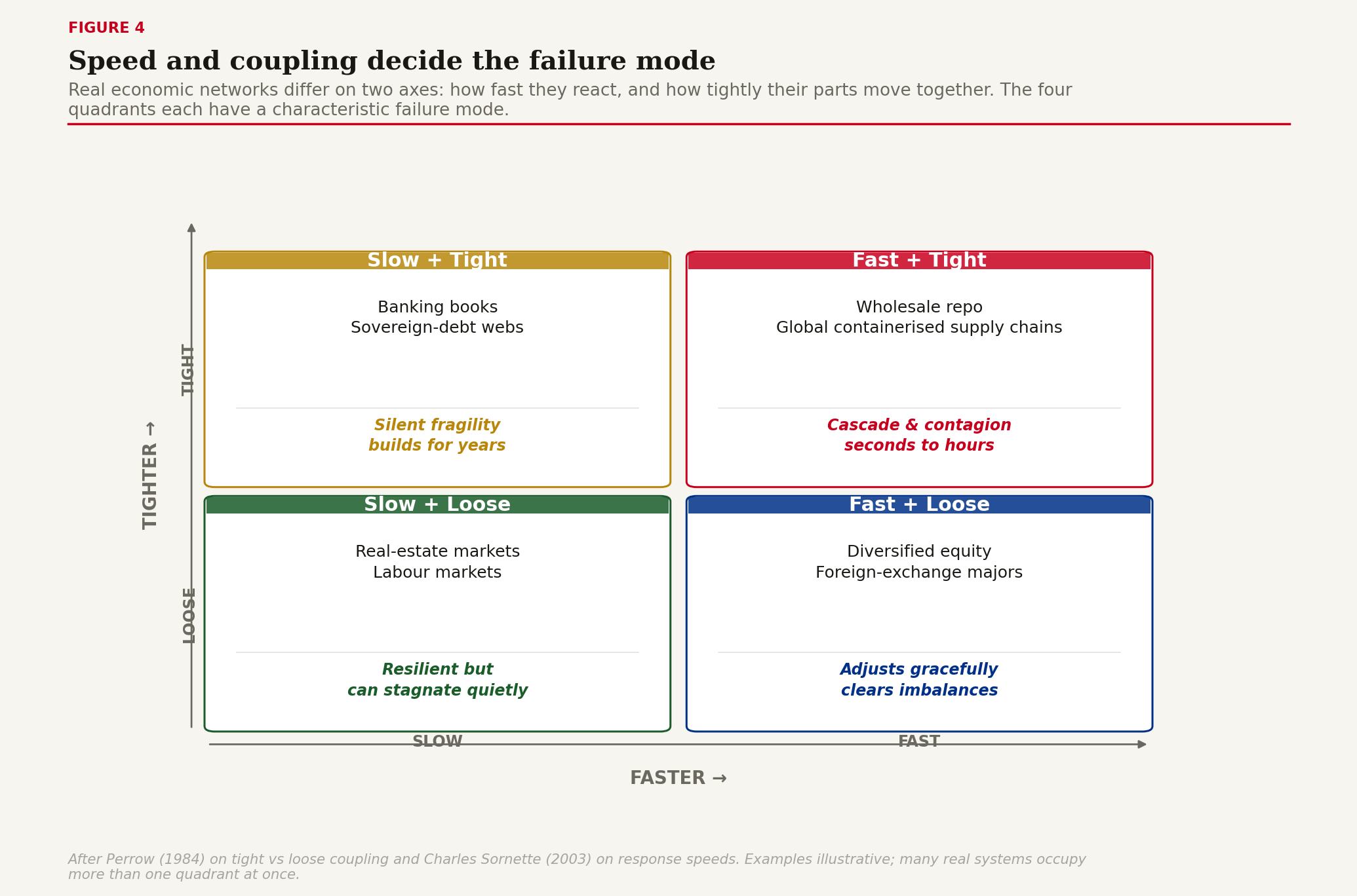
Figure 4: Tight versus loose coupling matrix. 2×2 of speed × coupling, with example domains and characteristic failure modes in each quadrant.
Part two: Distortions
What happens to the signal
Real transmission rarely delivers the signal undistorted. Four mechanisms account for almost everything that goes wrong on the way: amplification through multi-tier supply chains; contagion through belief propagation; phase transition at critical coupling; and non-linear threshold response.
The first is the supply-chain operations researcher's home territory. Jay Forrester noticed it in the 1950s and John Sterman formalized it in the 1989 Beer Distribution Game: a 10% demand pulse at the retail end becomes a much larger production whip upstream, with a phase lag of 8--10 weeks. The mechanism is straightforward --- each tier in the network optimizes its own inventory locally, with delay, and the optimization-with-delay amplifies. Each tier overshoots its target, the upstream tier sees the overshoot as a new demand pulse and overshoots its own response, and the signal becomes progressively detached from the underlying consumer demand it was supposed to track.
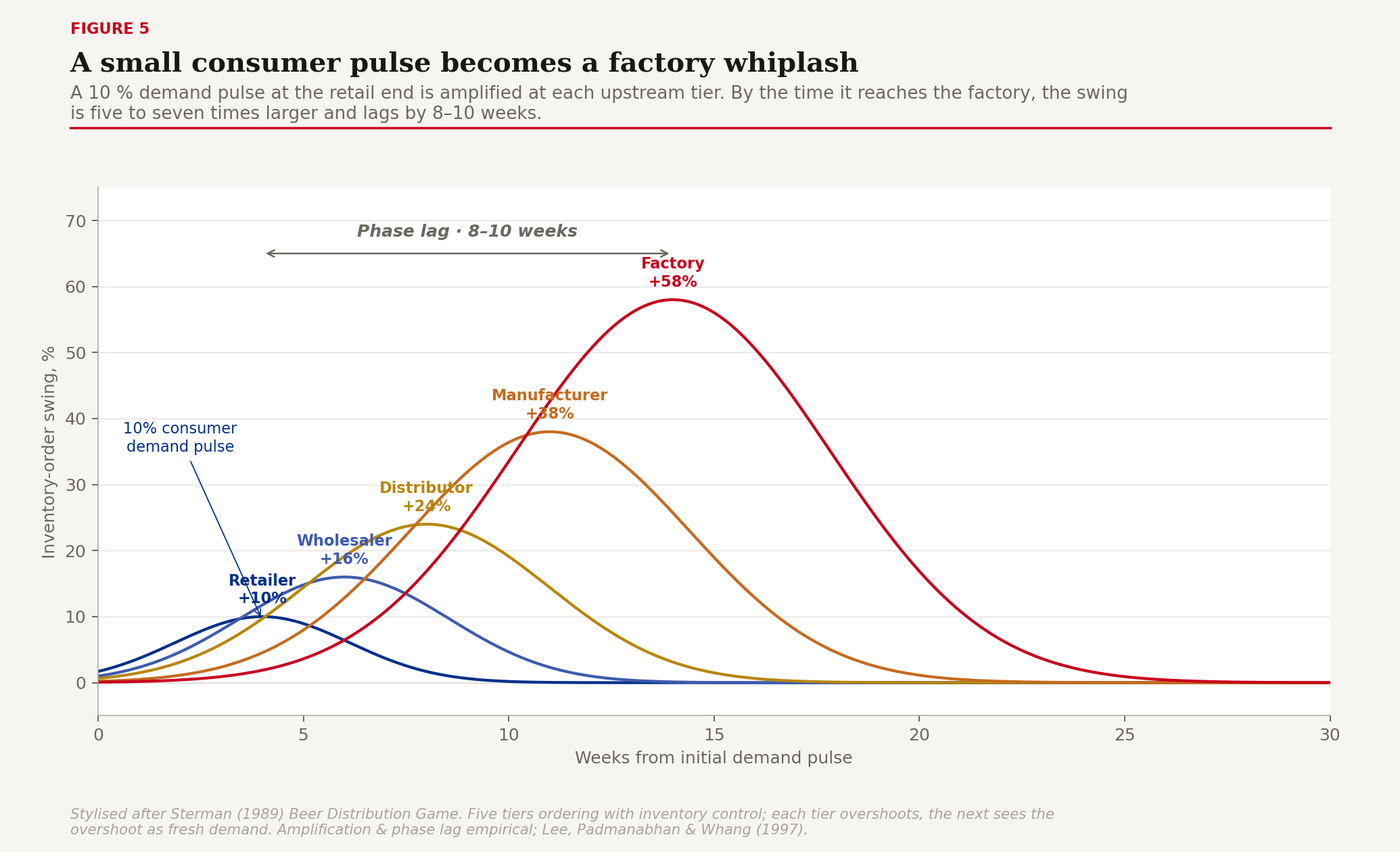
Figure 5: The bullwhip effect. Five tiers from consumer to factory, with the factory production curve showing 5--7× amplification and 8--10 week phase lag relative to a 10% consumer demand pulse.
The second mechanism is contagion. The epidemiologist's SIR model --- susceptible, infected, resolved --- was written for disease in 1927 and applies almost verbatim to beliefs. The control parameter is R₀, the reproduction number: how many new believers each existing believer infects on average. Below R₀ = 1, beliefs die out; above R₀ = 1, they spread to a large fraction of the population. The same curve describes meme stocks, bank runs, currency panics, and the adoption of any new economic narrative. Akerlof and Shiller's Animal Spirits (2009) made the analogy explicit; the math has been quietly waiting for it since 1927.
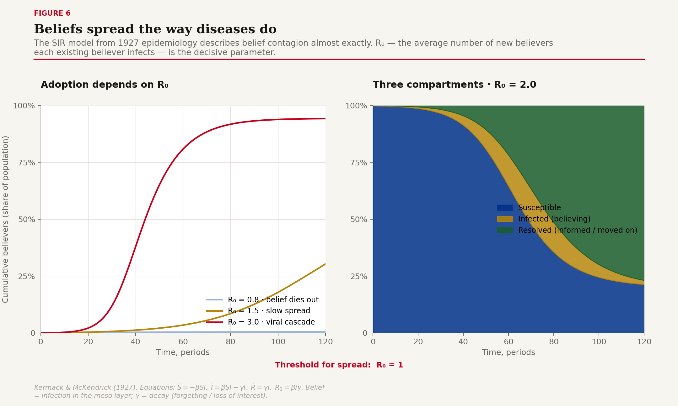
Figure 6: Beliefs spread like epidemics. Left: adoption curves at R₀ = 0.8, 1.5, 3.0. Right: SIR compartments through an R₀ = 2.0 epidemic. Ṡ = −βSI; İ = βSI − γI; Ṙ = γI; R₀ = β/γ.
The third mechanism is phase transition. The complex-systems physicist views the economy as a critical system: most of the time it is in the sub-critical regime where perturbations damp out, occasionally it is near the critical point where response is power-law, and during crises it crosses into the super-critical regime where cascades self-sustain. The dangerous regime is the narrow band just past the threshold, where small additional inputs produce disproportionately large outcomes. Spring 2008 lived just sub-critical. September 15, 2008 was the crossing. By the end of that week the system was deep in super-critical territory and every bilateral counterparty relationship in the wholesale funding market was being repriced in hours.
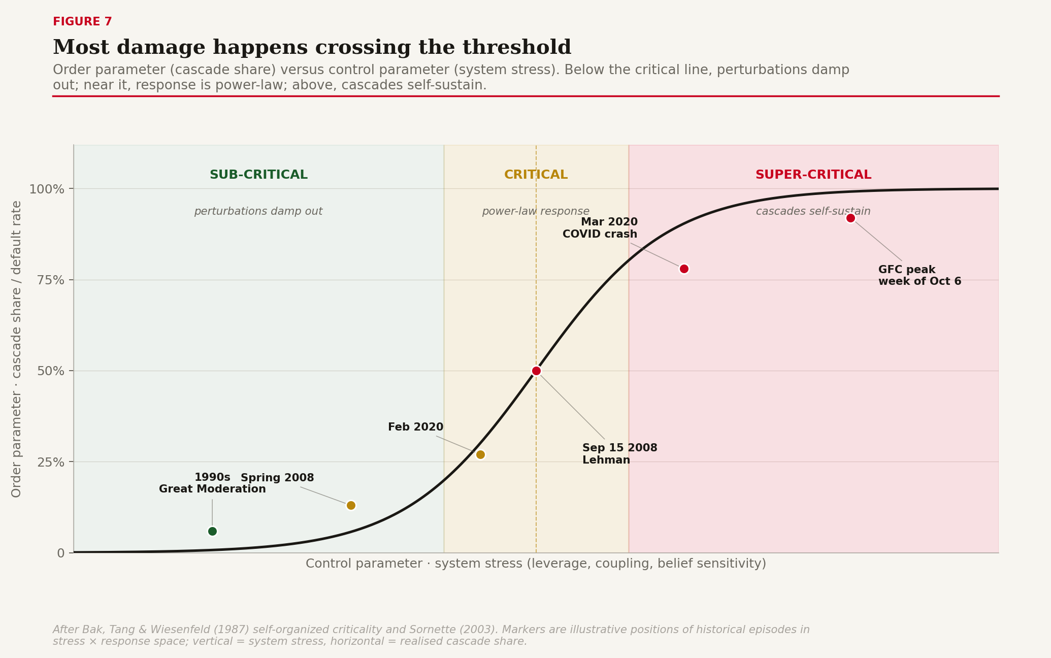
Figure 7: Phase transition. Order parameter (cascade share, default rate, panic intensity) versus control parameter (leverage, coupling, belief sensitivity). Sub-critical, critical, and super-critical zones with historical points marked.
The fourth mechanism is non-linear threshold response. Conventional macro often assumes a linear response --- a unit of policy produces a unit of behavior change, multipliers are constant, the Phillips curve is a line. Reality is S-shaped. There is a dead zone where the signal is too small to register (a 25 basis-point cut at the zero bound, an unread tweet, a credit easing nobody believes). There is an inflection zone where each unit of additional policy produces a large additional response (Volcker 1979--82 was almost the entire post-war American example of the inflection zone for monetary tightening). And there is a saturated zone where the response curve flattens and further policy has diminishing returns (the third round of quantitative easing after the first two have done most of the work).

Figure 8: Non-linear S-curve response. Three regimes: dead zone, inflection zone, saturated zone, contrasted with the linear (Phillips-curve) assumption.
Part three: Emergent field effects
What comes out
What the macro layer measures --- inflation, GDP, the credit cycle --- is not what is happening on the meso layer. The macro variables are emergent fields, statistical fingerprints of millions of decentralized decisions coordinated through the Shimmer. Treating them as primary objects rather than as the visible shadow of meso-layer activity is the most common diagnostic error in monetary economics.
Take inflation. There is no single price-setter called "inflation." Millions of firms decide independently each week whether to raise, hold, or cut their prices, based on their own costs, their own demand observations, and their own expectations about what others will do. The 2% reading that arrives in the CPI release is a statistical average of those decisions, weighted by consumption shares. What the central bank actually moves with a rate decision is not inflation itself, but the distribution of price-setting decisions across the population of firms --- a shift of the mean, a tightening of the variance, a damping of the long tail of large increases. The macro number is the emergent fingerprint.
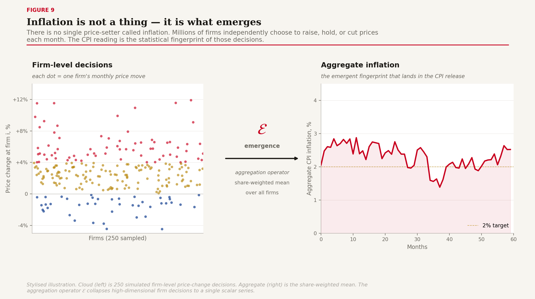
Figure 9: Inflation as emergence. Left: a cloud of local price-setting decisions, each firm raising or cutting by a different amount. Middle: the emergence operator. Right: the smooth aggregate inflation series that emerges from millions of such local decisions.
GDP is the same kind of object on a different axis. GDP is not a stock of value; it is a flow --- the rate at which value gradients get resolved through the network per unit time. The same physical economy with the same underlying capital stock and the same population can produce very different GDPs depending on whether gradients are being resolved fast or slow. A recession is not an economy with fewer gradients; it is an economy where existing gradients fail to resolve because trust has shortened, credit has tightened, or expectations have collapsed. A boom is the same gradients resolving faster. The implication for policy is that boosting GDP is about removing the frictions that prevent gradient resolution, not about creating new gradients out of thin air.
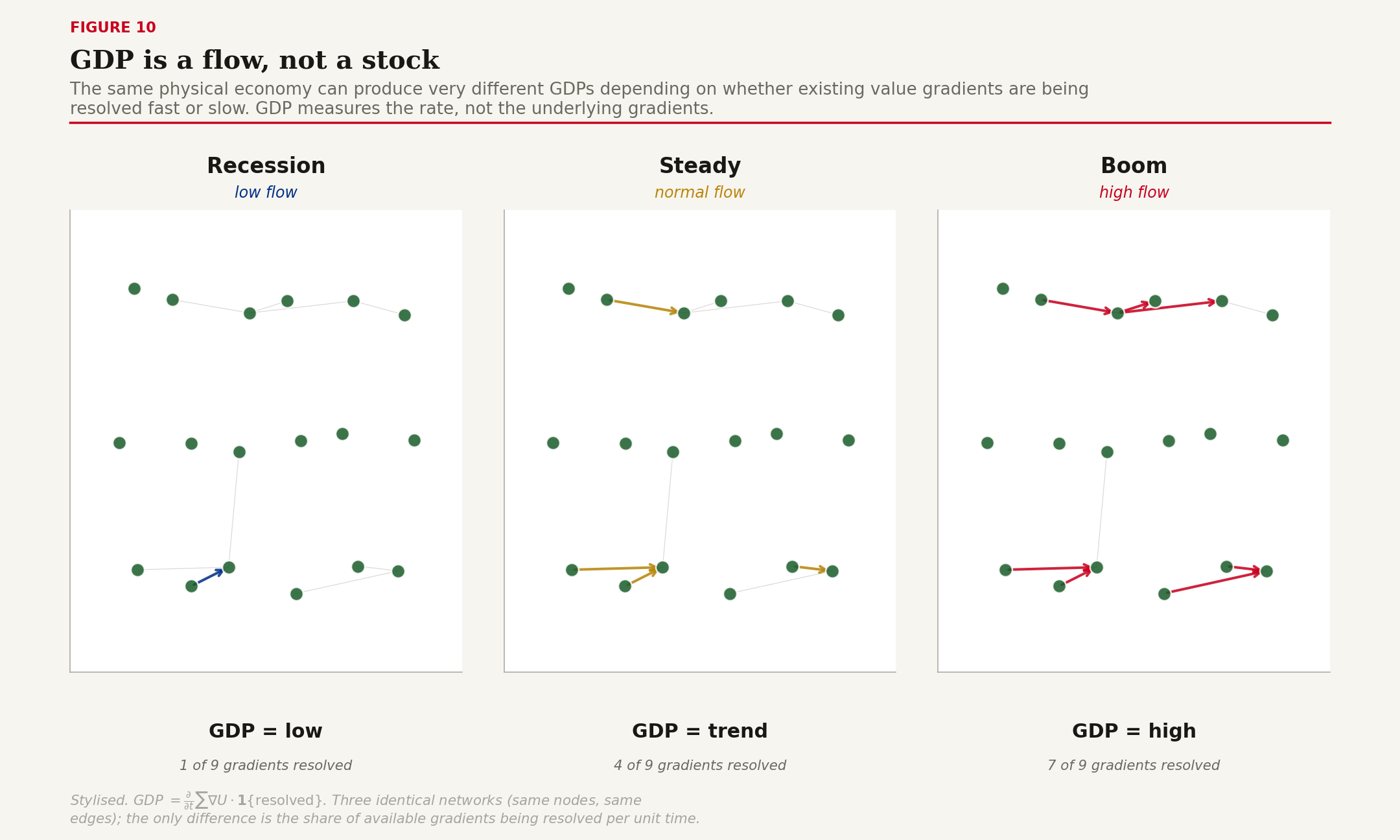
Figure 10: GDP as gradient-resolution rate. Three identical networks at different flow rates --- low / steady / high --- with the rate equation GDP = ∂/∂t Σ ∇U·1{resolved}.
The credit cycle is the third major emergent field, and it is the most consequential one for crisis dynamics. Base money (M0) is small and relatively stable; the credit aggregate sitting on top of it is roughly nine times larger and varies sharply with the network's willingness to extend and accept receivables. When the network is confident, credit expands and the realized GDP track is well above what the monetary base alone would support. When the network is fearful, credit contracts, and the monetary base often expands sharply (because the central bank is trying to compensate for the credit contraction) but the realized economy still shrinks because the multiplier has collapsed. The crucial point is that credit expansion and contraction is a meso-layer phenomenon --- it is the network's willingness to hold and extend receivables, not the central bank's reserve-creation activity, that moves the credit aggregate.
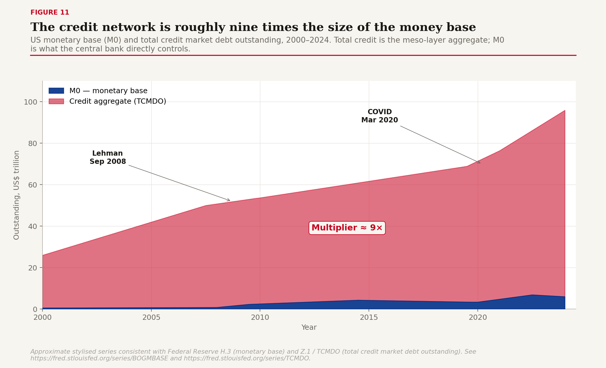
Figure 11: Credit network expansion and contraction. Stacked area chart of US M0 versus total credit, 2000--2024, with the 9× multiplier annotated and the 2008 GFC and 2020 COVID episodes marked.
Part four: Ten cases
The framework on history
A framework that does not predict observed outcomes is not a framework. The following ten cases were chosen MECE across the design space --- sudden vs slow, tight vs loose, policy vs private, monetary vs physical. Each illustrates a different transmission profile.
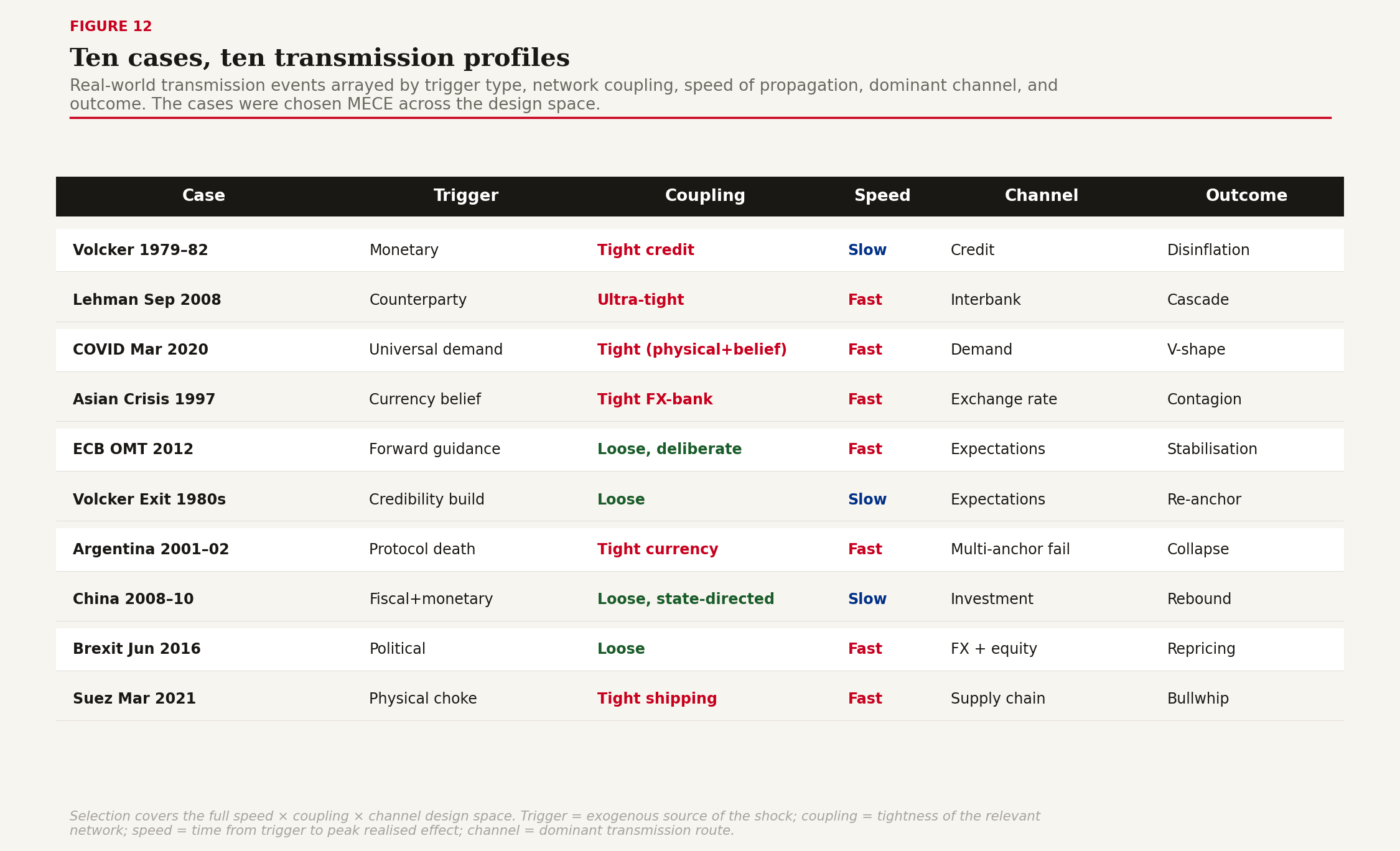
Figure 12: Ten transmission cases taxonomy table. Columns: trigger type, coupling, speed, channel, outcome.
Case 1: Volcker 1979--82
Sudden monetary shock, tight credit-channel coupling, slow real-economy response. The Federal Reserve under Paul Volcker raised the funds rate to 19% and held it there long enough to break inflation expectations. The credit channel was the binding constraint on transmission; bank lending standards tightened, the prime rate followed the funds rate, and the real economy slid into the deepest recession since the 1930s. Disinflation was achieved at substantial cost. The case demonstrates a slow successful transmission through a tightly coupled credit network.
Case 2: Lehman September 2008
Counterparty failure, ultra-tight coupling, instantaneous propagation. By the morning after Lehman's bankruptcy filing, overnight repo markets had frozen across every major dealer in the Western financial system. The transmission channel was the bilateral counterparty graph --- every dealer was a node, every overnight repo contract was an edge, and Lehman's removal from the graph triggered a cascade of margin calls and counterparty downgrades that propagated at the speed of risk-management software. The case is the canonical fast-tight cascade.
Case 3: COVID March 2020
Universal demand shock, tight coupling through both physical and expectations channels, near-instantaneous global propagation. The shock was simultaneous lockdowns across every major economy. Demand for travel, hospitality, and energy collapsed within days; supply chains stopped within weeks; the equity market lost a third of its value in five weeks. The Fed and Treasury response was unprecedented in size and speed, and the eventual recovery was V-shaped. The case demonstrates fast-tight transmission of a non-financial shock and the meso-layer mechanism of policy speed beating policy size.
Case 4: Asian crisis 1997
Currency-belief contagion, tight FX-and-banking coupling, fast regional propagation. The Thai baht devaluation in July 1997 triggered a contagion that propagated through the dollar-funded banking systems of Indonesia, Korea, and Malaysia in months. The transmission channel was the implicit dollar peg, which collapsed when the network's belief in the peg collapsed. The case is the canonical demonstration that currency arrangements live in the belief field, not in the reserves balance.
Case 5: ECB OMT July 2012
Pure forward guidance, deliberately loose coupling, fast belief response. Mario Draghi's three words --- "whatever it takes" --- collapsed the Spain--Germany sovereign spread by 200 basis points without a single euro of OMT actually being deployed. The mechanism was entirely through the expectations channel. The case is the most cost-effective transmission in modern monetary history per unit of policy action, and demonstrates that the credibility of an instrument matters more than its use.
Case 6: Volcker exit 1980s
Credibility build, loose coupling, slow steady decline. After the 1979--82 shock, the Fed under Volcker and then Greenspan built a new equilibrium: stable 2--3% inflation, anchored expectations, gradual unwinding of the high real-rate regime. The transmission was almost entirely through the expectations channel and took the better part of a decade. The case demonstrates that the meso layer can be re-anchored, but slowly.
Case 7: Argentina 2001--02
Protocol death, tight currency coupling, fast collapse. The corralito and pesification destroyed the credibility of the peso as a store of value. Dollarization de facto became the norm. The case is the canonical example of currency-protocol death, with the meso-layer mechanism being the simultaneous failure of the earnings anchor (collapsing real income), the taxation anchor (tax payments increasingly in barter or dollars), and the network anchor (acceptors switching protocols). Once all three anchors fail, no rate level restores the protocol.
Case 8: China 2008--10
Coordinated fiscal-plus-monetary stimulus, loose coupling through state-directed investment, slow but powerful pulse. The CNY 4 trillion stimulus package directed credit through the state-bank network into infrastructure investment. Transmission was slow (a year to fully manifest) but powerful (real GDP growth rebounded above 10%). The case demonstrates that loose-coupled networks can be steered effectively if the planner can write the directives directly into the network's wiring.
Case 9: Brexit June 2016
Political shock, loose coupling through the FX and equity channels, fast asset repricing. The unexpected referendum result triggered a one-day 8% sterling depreciation and persistent reduction in equity valuations of UK-exposed firms. The case demonstrates fast asset-channel transmission for a non-economic shock, with the real-economy effects taking much longer because the underlying trade and labor frictions had not yet changed.
Case 10: Suez March 2021
Physical supply-chain choke, tight coupling through global containerized shipping, fast amplification through the bullwhip mechanism. The Ever Given's six-day grounding triggered a container price spike that took 18 months to fully unwind, with knock-on inventory build-ups in 2021 and the famous "everything bubble" of consumer goods inventory in 2022. The case demonstrates that physical-network shocks transmit through exactly the same field-theoretic mechanism as monetary ones, with the bullwhip operator doing the amplification.
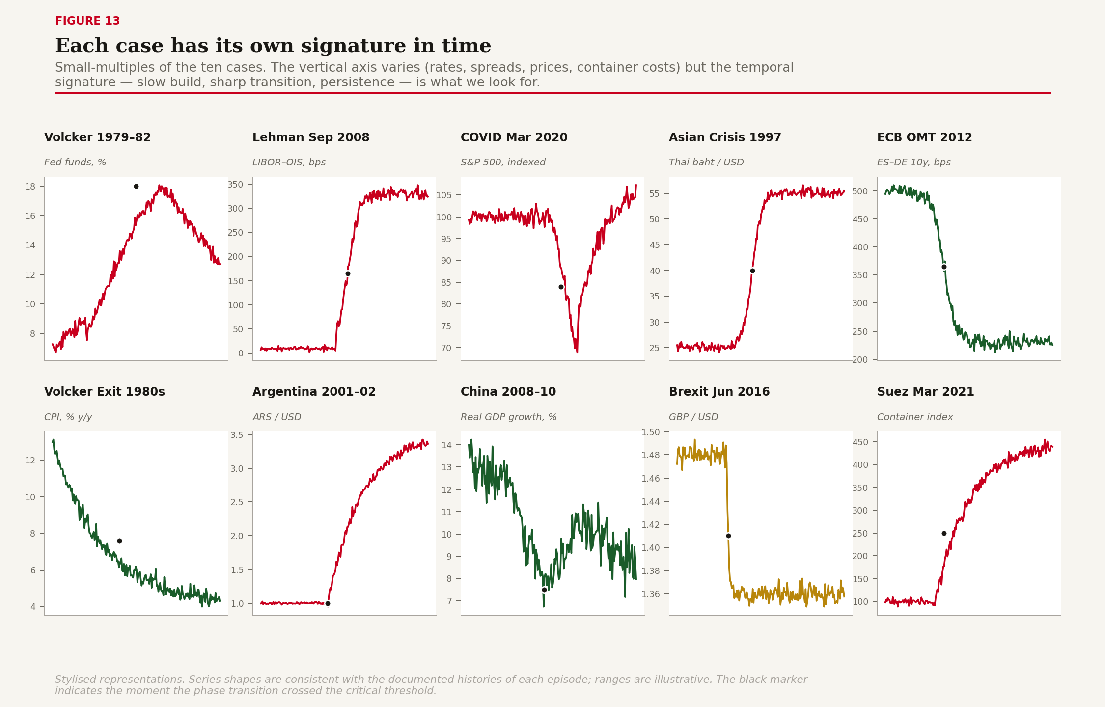
Figure 13: Ten transmission cases in time. Small multiples showing the characteristic phase-transition signature of each case in the relevant indicator series.
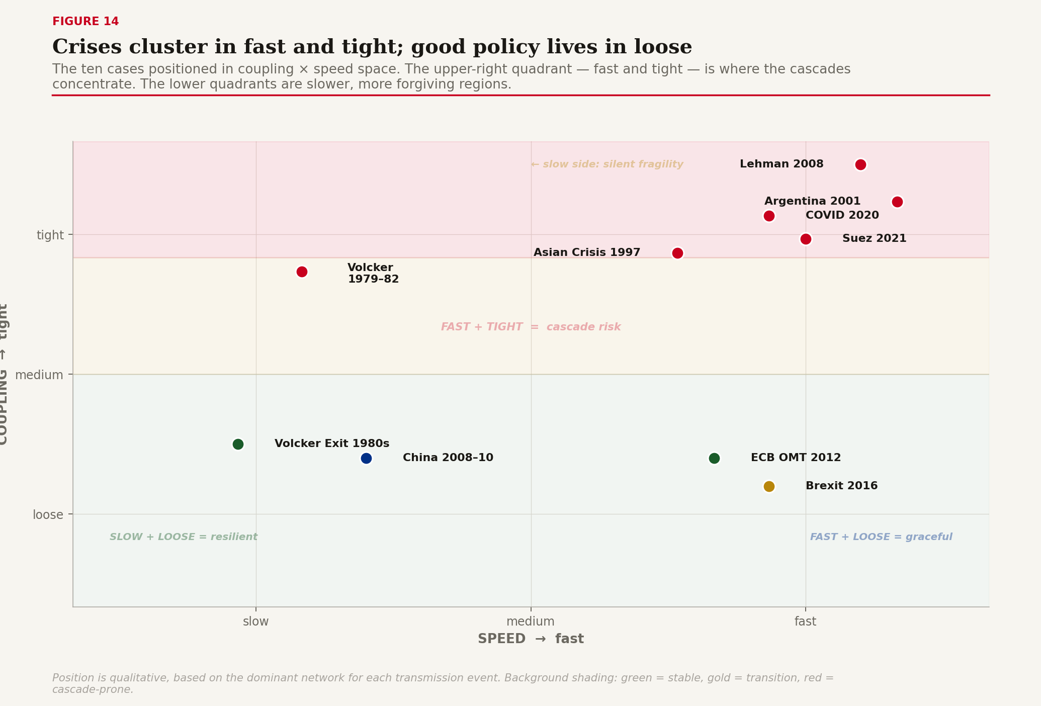
Figure 14: Phase diagram of transmission. Coupling × speed, with the ten cases plotted by their position in the design space. Crises cluster in fast-tight; successful policy interventions cluster in loose quadrants.
Six lessons for anyone sending a signal
Each lesson is a falsifiable claim derived from the ten cases.
One: Speed beats size. A small, fast signal reaching the right nodes outperforms a large, slow one. ECB's three-word OMT outperformed roughly €1 trillion of subsequent liquidity programs.
Two: Tight coupling equals cascade risk. When the network is tightly coupled, shocks propagate at light speed. The banking system in 2008 was so tightly coupled that Lehman's failure froze every overnight market by morning.
Three: Non-linearity at the threshold. Most damage happens crossing the phase boundary. The 25 basis points that takes you from sub-critical to super-critical looks identical to any other 25 basis points --- until it isn't.
Four: Bullwhip everywhere. Multi-tier networks amplify shocks. A 10% retail demand pulse becomes a 5--7× factory whip. The signal at the far end of the chain bears almost no resemblance to the signal at the start.
Five: Repetition beats announcement. Beliefs decay (λ \> 0). A single policy announcement is mostly forgotten in weeks. Effective central banking is repetition through a thousand speeches, minutes, and dot plots.
Six: The signal is the belief, not the rate. The Fed does not move inflation; it moves expectations about inflation. When the credibility channel is broken (Argentina, Turkey), no rate level restores transmission.
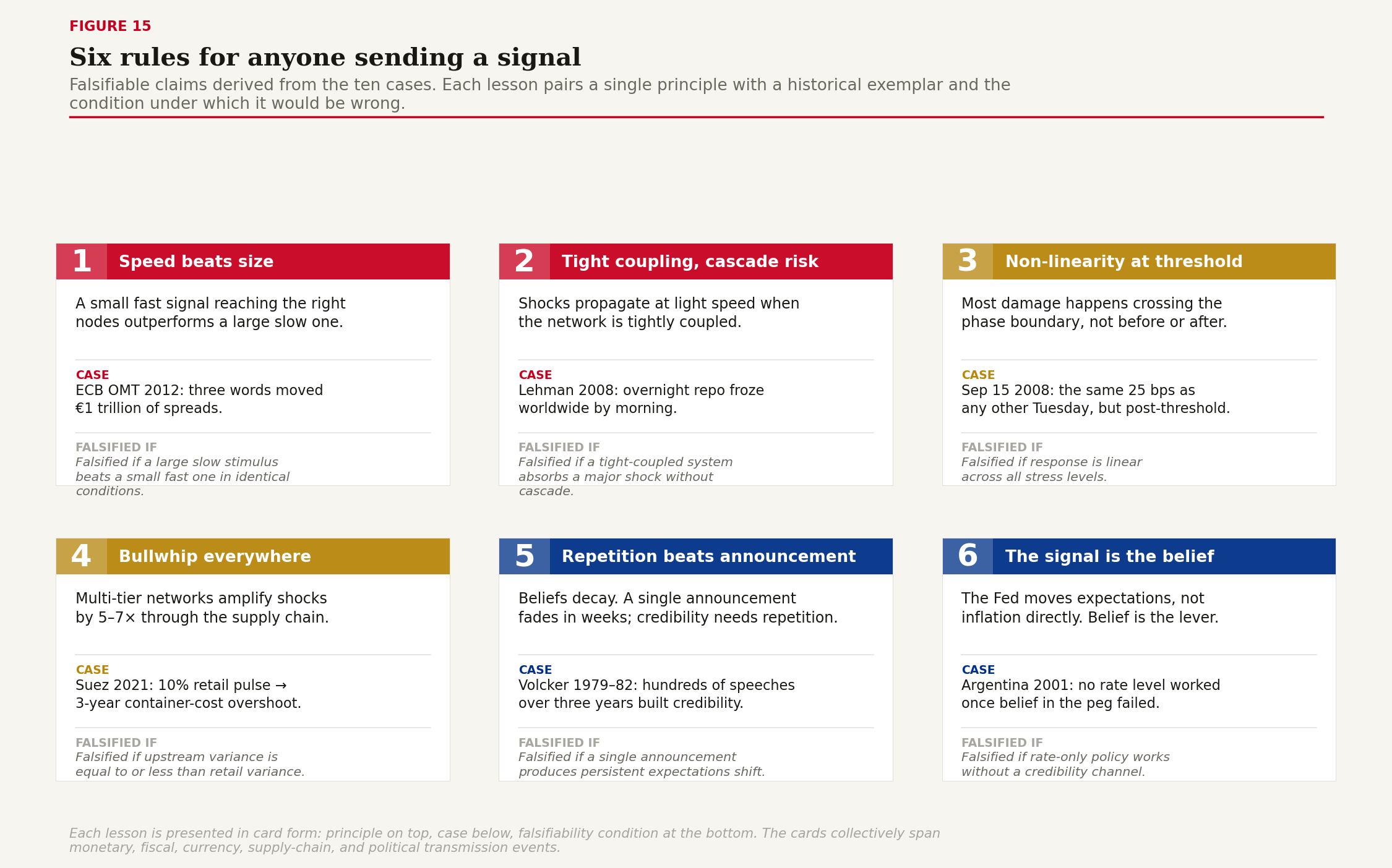
Figure 15: Six lessons map. Each lesson as a card with its key claim, the case it derives from, and the falsifiability condition.
Closing: Why the field view matters
Transmission is the central object of meso-economics. Every important monetary-policy question, every supply-chain stress, every contagion event, reduces to the same family of dynamics: a signal injected at one node, propagating through a network with measurable diffusion and decay, distorted by amplification, contagion, and non-linearity, emerging on the far side as an aggregate field effect.
The conventional macro framing treats transmission as a black box and works with input-output relationships fitted on past data. This is fine in stable periods and disastrous in regime changes, because the input-output mapping itself is a function of network topology and coupling --- and those change exactly when they matter most.
The meso-economic framing opens the black box. It makes transmission a measurable object with measurable parameters. It allows policy designers to ask not just "what rate should we set" but "through which network are we expecting the rate to travel, at what speed, with what coupling, against what background of beliefs." That richer question is what monetary policy in the 21st century needs to be capable of asking.
The molecules are real. The weather is real. But the climate --- that vast intersubjective field of expectations and beliefs and protocols, slower than a trade and faster than a national-accounts revision --- is just as real, and most of the things you care about in an economy happen there.
Sources and further reading
Akerlof, G. & Shiller, R. (2009). Animal Spirits: How Human Psychology Drives the Economy. Princeton University Press.
Akerlof, G., Dickens, W. & Perry, G. (1996). The Macroeconomics of Low Inflation. Brookings Papers on Economic Activity 1996(1).
Anderson, P. W. (1972). More Is Different. Science 177(4047): 393--396.
Anderson, R. M. & May, R. M. (1991). Infectious Diseases of Humans: Dynamics and Control. Oxford University Press.
Bak, P., Tang, C. & Wiesenfeld, K. (1987). Self-organized criticality: An explanation of the 1/f noise. Physical Review Letters 59(4).
Barabási, A. L. & Albert, R. (1999). Emergence of scaling in random networks. Science 286(5439): 509--512.
Bernanke, B. & Gertler, M. (1995). Inside the Black Box: The Credit Channel of Monetary Policy Transmission. Journal of Economic Perspectives 9(4).
Borio, C. (2014). The financial cycle and macroeconomics: What have we learnt? Journal of Banking & Finance 45.
Draghi, M. (2012). Speech at the Global Investment Conference, London, 26 July. "Whatever it takes."
Glosten, L. & Milgrom, P. (1985). Bid, ask and transaction prices in a specialist market with heterogeneously informed traders. Journal of Financial Economics 14.
Gogerty, N. & Johnson, P. (2018). Currency Is a Network Protocol: Network Capital Theory and 95 Currencies. SSRN 3281845. https://ssrn.com/abstract=3281845
Kahneman, D. (2011). Thinking, Fast and Slow. Farrar, Straus & Giroux.
Kermack, W. & McKendrick, A. (1927). A contribution to the mathematical theory of epidemics. Proceedings of the Royal Society A 115.
Kindleberger, C. (1978). Manias, Panics, and Crashes: A History of Financial Crises.
Kyle, A. (1985). Continuous auctions and insider trading. Econometrica 53(6).
Lee, H., Padmanabhan, V. & Whang, S. (1997). Information distortion in a supply chain: The bullwhip effect. Management Science 43(4).
Mishkin, F. (1995). Symposium on the Monetary Transmission Mechanism. Journal of Economic Perspectives 9(4).
Perrow, C. (1984). Normal Accidents: Living with High-Risk Technologies. Basic Books.
Reinhart, C. & Rogoff, K. (2009). This Time Is Different: Eight Centuries of Financial Folly. Princeton University Press.
Sargent, T. (1982). The Ends of Four Big Inflations. In Hall (ed.) Inflation: Causes and Effects.
Shannon, C. (1948). A Mathematical Theory of Communication. Bell System Technical Journal 27.
Sornette, D. (2003). Why Stock Markets Crash: Critical Events in Complex Financial Systems. Princeton University Press.
Sterman, J. (1989). Modeling managerial behavior: Misperceptions of feedback in a dynamic decision making experiment. Management Science 35(3).
Sterman, J. (2000). Business Dynamics: Systems Thinking and Modeling for a Complex World.
Strogatz, S. (2003). Sync: The Emerging Science of Spontaneous Order. Hyperion.
Watts, D. & Strogatz, S. (1998). Collective dynamics of small-world networks. Nature 393.